
Industrial Engineering
Frontiers in Industrial Engineering ·
Volume 3 - 2025 | https://doi.org/10.3389/fieng.2025.1620422
Hybrid heuristic approach for generalized police officer patrolling problem
- Fumito Kudo1
- Hiroaki Tohyama2
- Masaki Tomisawa2*corresponding author
- 11 Department of Life Science and Informatics, Graduate School of Engineering, Maebashi Institute of Technology, Maebashi, Gunma, Japan
- 22 Department of Life Engineering, Faculty of Engineering, Maebashi Institute of Technology, Maebashi, Gunma, Japan
Abstract
In urban areas with many commercial facilities, patrolling by police officers or security guards is essential for crime prevention, in addition to the use of surveillance cameras. To address the challenge of planning effective patrol routes, Tohyama and Tomisawa introduced the Police Officer Patrolling Problem (POPP), an arc routing problem that allows for visual monitoring from intersections and is proven to be NP-complete. Building on this work, we propose the Generalized POPP (GPOPP), a more realistic bi-objective combinatorial optimization model. This model simultaneously minimizes the total patrol route length and maximizes the coverage of surveillance areas. The contributions of this paper are threefold: (1) we formulate the GPOPP by incorporating practical constraints, such as mandatory patrolling of high-security roads and visibility-based coverage from intersections; (2) we develop a novel hybrid heuristic method that combines a multi-objective evolutionary algorithm (MoEA-HSS) with an improved Jaya algorithm to solve the GPOPP effectively; and (3) we conduct comprehensive computational experiments using benchmark instances to evaluate the effectiveness and competitiveness of the proposed method. These contributions demonstrate the practicality and efficiency of our approach for addressing realistic urban patrolling problems.
Keywords
1 Introduction
In the fields of information engineering and science, to solve various social and economic problems, these problems are generally structured as mathematical models, and solutions are found using algorithms that are suited to that structure. Many of these problems are modeled using discrete graphs, and there are many studies on them.
One of the problems modeled by discrete graphs is the routing problem. Routing problems are classified as node routing problems (NRPs), which traverse the nodes of a graph, and arc routing problems (ARPs), which traverse the edges (or arcs). A typical NRP is the traveling salesperson problem (TSP). The TSP is a problem that involves finding the minimum-cost route that visits every vertex exactly once. The vehicle routing problem (VRP) (Dantzig and Ramser, 1959) is a generalization of the TSP. This problem involves planning transportation from a distribution center to multiple customers using trucks or other transportation methods. Both the TSP and VRP are NP-hard; thus, evolutionary algorithms, such as genetic algorithms (GAs), have been studied (Elatar et al., 2023).
The most famous ARP is probably the Euler circuit problem. This problem determines whether there exists a circuit that traverses all edges exactly once for a given graph, and this problem is solvable in polynomial time. The Chinese postman problem (CPP) (Mei-Ko, 1962), which is a generalization of the Euler circuit problem, involves determining whether a tour exists for a post officer in a given area within a given amount of time that starts and ends at the post office. The post officer must traverse every street in the area at least once; however, they may traverse any street several times. The CPP on undirected or directed graphs can be solved in polynomial time (Edmonds and Johnson, 1973). Papadimitriou (1976) showed that the CPP on mixed graphs is NP-complete. Mixed graphs represent realistic situations in urban areas with both two- and one-way streets. The rural postman problem (RPP) is a generalization of the CPP with a given set of edges that must be traversed by a post officer. This problem considers the fact that, in rural areas, not every street has a delivery destination. Lenstra and Rinnooy-Kan (1976) and Lenstra and Rinnooy-Kan (1981) showed that the optimization version of the RPP on undirected or directed graphs is NP-hard. The capacitated ARP (CARP) is an ARP corresponding to the VRP, which belongs to the NRP. The CPP, RPP, and CARP correspond to mathematical models of real social problems such as postal delivery, delivery planning, snow shoveling, and garbage collection. Finding exact solutions for the CPP and RPP optimization problems is intractable, along with the TSP and VRP; thus, various heuristic methods have been proposed for these problems. Recent examples include methods using GAs (Gil-Gala et al., 2023), the Tabu search algorithm (Tang et al., 2024), and ant colony optimization (Sgarro and Grilli, 2024).
Police patrols play a crucial role in preventing crimes and accidents, thereby ensuring public safety within their jurisdictions. Recent studies such as (Kim et al., 2023; Dewinter et al., 2020; Samanta et al., 2022) have proposed methods for optimizing patrol routes. These approaches primarily employ heuristic algorithms to generate efficient patrol routes for multiple officers operating within the shared area.
Recently, Tohyama and Tomisawa (2022) proposed the police officer patrol problem (POPP) as a mathematical model of the patrolling route problem of police officers (or security guards), and showed that the decision problem is NP-complete (Tohyama and Tomisawa, 2022). Patrolling areas generally include one- and two-way streets; thus, the POPP is modeled using a mixed graph. At each intersection, police officers may conduct security checks visually even if they do not traverse the streets connecting to it. If the POPP is considered a CPP model, it is necessary to find a patrolling route that traverses all streets. The POPP model allows some streets to conduct visual security checks without traversing, making it possible to find more efficient patrolling routes. In addition, Tomisawa and Tohyama showed that the POPP on weighted digraphs is NP-complete (Tomisawa and Tohyama, 2024).
In this study, we introduce the generalized POPP (GPOPP) as a model to adapt the POPP to more realistic patrolling routes by police officers. The POPP model requires that all areas be guarded. However, in reality, some streets require security because important facilities are located there, and some roads do not necessarily require security (Chainey et al., 2021). In addition, there are cases where a patrolling route needs to be found that can be patrolled within a given time. Therefore, we define the GPOPP as an optimization problem with the following two objectives. The first objective is to find the shortest patrolling route among the routes that traverse all high-security streets. The second objective is to find a patrolling route that guards as large a given area as possible (maximizes coverage).
Many GAs have been proposed to solve multi-objective problems (Deb et al., 2002; Sardinas et al., 2006; Pizzuti, 2009; Ghoseiri and Ghannadpour, 2010; Aiello et al., 2012; Akyurt et al., 2015; Yu et al., 2015; Lu et al., 2019). The hybrid sampling strategy based multi-objective evolutionary algorithm (MoEA-HSS) (Zhang et al., 2014) is based on a hybrid sampling strategy that combines a vector-valued GA (VEGA) (Schaffer, 2014) and a sampling strategy according to the Pareto dominating and dominated relationship-based fitness function (PDDR-FF) (a goodness-of-fit function based on Pareto dominance–dominance relations). The MoEA-HSS has demonstrated effectiveness for several problems. The Jaya algorithm (Rao, 2016) is a meta-heuristic algorithm with a very simple structure based on the concept that solutions obtained for a particular problem progress toward the best solution and avoid the worst solution. We propose a hybrid heuristic approach that combines the MoEA-HSS with an improved Jaya algorithm, and demonstrate its effectiveness through numerical experiments.
The remainder of this paper is organized as follows. In Section 2, we formally define the Generalized Police Officer Patrolling Problem (GPOPP) and present the necessary graph-theoretical concepts. Section 3 provides a mathematical formulation of the GPOPP as a bi-objective optimization problem. In Section 4, we describe the proposed hybrid heuristic method that combines the MoEA-HSS and an improved Jaya algorithm. Section 5 presents the results of the numerical experiments conducted to evaluate the performance of the proposed method. Finally, Section 6 concludes the paper and discusses potential directions for future research.
2 Generalized police officer patrolling problem (GPOPP)
In this study, we introduce a bi-objective problem that can be applied to more realistic problems based on the POPP, which is NP-complete edge routing decision problem, and propose a heuristic algorithm to solve the problem. One police officer (or security guard or robot) is assigned to a security area, and each officer patrols his/her assigned area. Each street through which a police officer is traversed during a patrol is considered guarded. In addition, except for streets with important facilities, police officers are allowed to visually confirm each street adjacent to an intersection without traversing it. The GPOPP is a bi-objective optimization problem with the following two objectives: One is to find the patrolling route with the shortest length, and the other is to find the route with the largest guarded area. Here, we note that all high-security streets must be traversed. In this section, we define the notion in graph theory necessary to formulate the GPOPP.
Throughout this paper, let N = { 1 , 2 , 3 , ⋯ } be the set of all natural numbers. Let I k = { 0 , 1 , 2 , ⋯ , k − 1 } and I k + = { 1 , 2 , 3 , ⋯ , k } for each k ∈ N. Let G = ( V , E , A ) be a connected simple mixed graph, where V is the set of vertices, E is the set of undirected edges and A is the set of arcs. Hereafter, the number of vertices in G is denoted as n and fixed to V = { 1,2 , … , n }. Here, we denote an undirected edge by { u , v } and an arc by ( u , v ). The term “edge” refers to either an undirected edge or an arc, denoted by ⟨ u , v ⟩. Thus, if ⟨ u , v ⟩ is an undirected edge, ⟨ u , v ⟩ = ⟨ v , u ⟩; if it is an arc, ⟨ v , u ⟩ ∉ A.
Let m ∞ be a sufficiently large positive integer. Then, let d be a function from V 2 to N satisfying the following conditions: for all u, v ∈ V
- 1. d ( u , v ) = d ( v , u ),
- 2. ⟨ u , v ⟩ ∈ E ∪ A or ⟨ v , u ⟩ ∈ E ∪ A ⇒ d ( u , v ) < m ∞,
- 3. ⟨ u , v ⟩, ⟨ v , u ⟩ ∉ E ∪ A ⇒ d ( u , v ) = m ∞.
Here, d ( u , v ) denotes the distance between u and v if there exists an edge ⟨ u , v ⟩ (or ⟨ v , u ⟩). For convenience, d ( u , v ) = m ∞ when there is no edge between u and v.
Let H be a subset of E ∪ A. We consider that there exist important facilities on each edge in H that must be stopped at. Each edge in H is considered a high-security edge. A sequence s: v 0, v 1, v 2, ⋯, v k of vertices is considered a patrolling route on G if the following conditions hold:
- 1. The sequence s is a walk. That is, ⟨ v i , v i + 1 ⟩ ∈ E ∪ A for each i ∈ I k.
- 2. All edges in H are on s. That is, if { u , v } ∈ H, there exists i ∈ I k satisfying u = v i and v = v i + 1 or u = v i + 1 and v = v i. If ( u , v ) ∈ H, there exists i ∈ I k satisfying u = v i and v = v i + 1.
- 3. v k = v 0. That is, the walk s is closed.
The length L ( s ) of a patrolling route s is the total sum of the distances of all edges on s and is calculated as follows:
L s = ∑ i = 0 k − 1 d v i , v i + 1 .
For a patrolling route s, let V s = { v i ∈ V | i ∈ I k } and E s = { ⟨ v i , v i + 1 ⟩ ∈ E ∪ A | i ∈ I k }. Here, V s denotes the set of vertices on s, and E s denotes the set of edges traversed in s. Let ⟨ u , v ⟩ be an edge of G. If u ∈ V s or v ∈ V s, the edge is considered guarded. In particular, if ⟨ u , v ⟩ ∈ E s, said the edge is considered guarded by traversing; otherwise, if exactly one vertex of u and v is in V s, the edge is considered guarded by visual confirmation.
Let E s g = { ⟨ u , v ⟩ ∈ E ∪ A | u ∈ V s or v ∈ V s } be a set of edges guarded by a patrolling route s. Then, the total sum of the distances of all edges guarded by s is denoted as ∑ ⟨ u , v ⟩ ∈ E s g d ( u , v ). The total sum of the distances of all edges of G is denoted as ∑ ⟨ u , v ⟩ ∈ E ∪ A d ( u , v ); thus, the covered ratio c o v ( s ) of G by s is defined as follows:
c o v s = ∑ 〈 u , v 〉 ∈ E s g d u , v ∑ 〈 u , v 〉 ∈ E ∪ A d u , v − 1 .
Similarly, c o v ̄ ( s ) = 1 − c o v ( s ) is called the noncovered ratio of G by s. For any patrolling route s of G, 0 < c o v ( s ) ≤ 1 and 0 ≤ c o v ̄ ( s ) < 1 holds.
An example of a patrolling route for a mixed graph is illustrated in Figure 1. The red edges represent high-security edges, and the blue line indicates a patrolling route. The green area is guarded by this patrolling route. In particular, the green area not on the patrolling route is guarded by visual confirmation. The graph shown in Figure 1 has 60 vertices and 104 edges. Let us assume that the distance between any two vertices is one. Then, the length of the patrolling route is 44. The total sum of the distances of the guarded edges is 84, and the covered and noncovered ratios are 0.808 and 0.192, respectively.

Let v i ( i ∈ I k ) be a vertex on a patrolling route s: v 0, v 1, v 2, ⋯, v k of a mixed graph G = ( V , E , A ). If ⟨ v i − 1 , v i ⟩, ⟨ v i , v i + 1 ⟩ ∉ H and ⟨ v i − 1 , v i + 1 ⟩ ∈ E ∪ A, then the sequence s ′: v 0, v 1, v 2, ⋯, v i − 1, v i + 1, ⋯, v k − 1, v k by removing v i from s is also a patrolling route of G (In the case i = 0, s ′: v 1, v 2, v 3, ⋯, v k − 1, v 1 is a patrolling route if ⟨ v k − 1 , v k ⟩, ⟨ v 0 , v 1 ⟩ ∉ H and ⟨ v k − 1 , v 1 ⟩ ∈ E ∪ A). Some edges guarded by visual confirmation from v i on s may not be guarded on s ′, although two edges removing from s are guarded by visual confirmation. That is, c o v ̄ ( s ) ≤ c o v ̄ ( s ′ ) holds. On the other hand, the increase or decrease in the length of the sequence v 0, v 1, v 2, ⋯, v k does not determine the increase or decrease in the length of the patrolling route. That is, L ( s ′ ) ≤ L ( s ) holds if the triangle inequality d ( v i − 1 , v i + 1 ) ≤ d ( v i − 1 , v i ) + d ( v i , v i + 1 ) (d ( v k − 1 , v 1 ) ≤ d ( v k − 1 , v k ) + d ( v 0 , v 1 ) in the case i = 0) is satisfied, otherwise, L ( s ) ≤ L ( s ′ ) holds.
3 Formulation
The GPOPP is a bi-objective optimization problem that obtains a patrolling route with the shortest length and the lowest noncovered ratio for a given connected simple mixed graph G = ( V , E , A ), a set H ⊆ E ∪ A of high-security edges, and a distance function d : V 2 → Z +. The parameters n, c u , v, h u , v, and d u , v for the GPOPP are defined as follows:
- (i) n: number of vertices.
- (ii) c u , v = 1 , if ⟨ u , v ⟩ ∈ E ∪ A , 0 , otherwise .
If G has an undirected edge { u , v }, c u , v = c v , u = 1; if G has an arc ( u , v ), c u , v = 1 and c v , u = 0.
- (iii) h u , v = 1 , if ⟨ u , v ⟩ ∈ H or ⟨ v , u ⟩ ∈ H , 0 , otherwise .
Note that h u , v = h v , u = 1 even if ⟨ u , v ⟩ is an arc in H.
- (iv) d u , v = d ( u , v ) for each ( u , v ) ∈ V 2.
- (v) c u , v ′ = 1 , if c u , v + c v , u > 0 , 0 , otherwise .
In other words, c u , v ′ = 1 when there is an edge that has endpoints u and v; c u , v ′ = 0 when there is no edge between them in the mixed graph G. c u , v ′ is immediately obtained from c u , v.
The decision variables for the GPOPP are x u , v and y u , v. The decision variable x u , v represents the number of times the edge ⟨ u , v ⟩ is traversed from u to v. If there exists no edge between u and v, x u , v = 0. The decision variable y u , v is expressed as follows:
- (vi) y u , v = 1 2 , if ∑ k = 1 n x u , k > 0 and ∑ k = 1 n x v , k > 0 , 1 , if ∑ k = 1 n x u , k > 0 and ∑ k = 1 n x v , k = 0 , 0 , otherwise .
We remark that ∑ k = 1 n x u , k is strictly positive if and only if the vertex u is in V s. Thus, y u , v = y v , u = 1 2 when both u and v are on s; y u , v = 1 and y v , u = 0 when u is on s even though v is not on s. Note that y u , v = y v , u = 1 2 does not mean that ⟨ u , v ⟩ or ⟨ v , u ⟩ are in E s. Then, ∑ u = 1 n ∑ v = 1 n c u , v ′ d u , v y u , v denotes the total length of edges guarded by the patrolling route s.
Let x = ( x 1,1 , x 1,2 , ⋯ , x n , n ) be an n 2-tuple of nonnegative integers. The mathematical model for the GPOPP is formulated as follows:
minimize f 1 x = ∑ u = 1 n ∑ v = 1 n d u , v x u , v , minimize f 2 x = 1 − ∑ u = 1 n ∑ v = 1 n c u , v ′ d u , v y u , v ∑ u = 1 n − 1 ∑ v = u + 1 n c u , v ′ d u , v − 1 .
The objective function f 1 is the function that minimizes the total length of the patrolling route, and f 2 is the function that minimizes the noncovered ratio.
The following constraints must be satisfied: where V x = u ∈ V ∑ v = 1 n x u , v > 0 is the same as V s defined in the previous section. Equation 1: The number of times to directly traverse from u to v is nonnegative. Equation 2: If there exists no edge between u and v or even if there exists an arc from v to u, it is not possible to directly traverse from u to v. Equation 3: The edge ⟨ u , v ⟩ (or ⟨ v , u ⟩) must be traversed if it is a high-security edge. Equation 4: For any vertex u, the number of times traversed from other vertices to u is the same as the number of times traversed from u to other vertices.
x u , v ≥ 0 ∀ u , v ∈ V , (1)
c u , v = 0 ⇒ x u , v = 0 ∀ u , v ∈ V , (2)
h u , v = 1 ⇒ x u , v + x v , u > 0 ∀ u , v ∈ V , (3)
∑ v = 1 n x v , u = ∑ v = 1 n x u , v ∀ u ∈ V , (4)
W ≠ ϕ ∧ W ≠ V x ⇒ ∑ u ∈ W ∑ v ∉ W x u , v > 0 ∀ W ⊆ V x , (5)
Suppose that x does not satisfy Equation 5. Then, there exists a nonempty proper subset W of V x that satisfies ∑ u ∈ W ∑ v ∉ W x u , v = 0. This means that any edge ⟨ u , v ⟩ incident to u ∈ W and v ∈ V x − W is not traversed; therefore, x represents two or more separate walks. In other words, based on Equation 5, the patrolling route is a continuous closed walk.
The notation used in formulating the mathematical programming model for GPOPP is summarized as follows:
- Parameters
- c u , v 1 if ⟨ u , v ⟩ ∈ E ∪ A, 0 otherwise
- c u , v ′ 1 if ⟨ u , v ⟩ ∈ E ∪ A or ⟨ v , u ⟩ ∈ E ∪ A, 0 otherwise
- d u , v same as d ( u , v )
- h u , v 1 if ⟨ u , v ⟩ ∈ H or ⟨ v , u ⟩ ∈ H, 0 otherwise
- n number of vertices
- Decision variables
- x u , v number of traversing from u to v
- y u , v 1 2 if both u , v on s, 1 if only one of u or v is on s 0 otherwise,
- Objective functions
- f 1 minimize the length of the patrolling route L ( s )
- f 2 minimize the length of the non-covered ratio c o v ̄ ( s )
4 Proposed methods
4.1 Framework
The GPOPP requires two conflicting objectives to be considered simultaneously: minimizing the total length of the patrolling route and minimizing its noncoverage ratio. Many Pareto-optimal solutions with incomparable qualities must be generated for the decision-maker. In this section, we introduce a hybrid heuristic approach based on the MoEA-HSS and the improved Jaya algorithm for the GPOPP.
The MoEA-HSS is based on a hybrid sampling strategy that combines the VEGA and a sampling strategy according to the PDDR-FF. The sampling strategy of the VEGA is a natural extension of simple GAs in the sense that the individuals are divided and reproduced independently according to each objective function. It prefers the edge region of the Pareto front with less time complexity, and the qualities of the solution are not good because of the selection bias. Conversely, the PDDR-FF-based sampling strategy tends to converge toward the central area of the Pareto front. The combination of these two mechanisms is expected to maintain both the convergence rate and distribution performance. The Jaya algorithm modifies a given individual to move closer to the best solution and away from the worst solution based on the best and worst candidates in the population. The Jaya algorithm is expected to accelerate the convergence rate.
The main framework of the proposed method is shown in Figure 2. The assemblage of chromosomes in each generation t is divided into two groups A ( t ) and P ( t ). A ( t ) and P ( t ) are called Archive and Population, respectively. The Pareto solution set update shown in the figure follows the same procedure as in the MoEA-HSS (Zhang et al., 2014) framework.
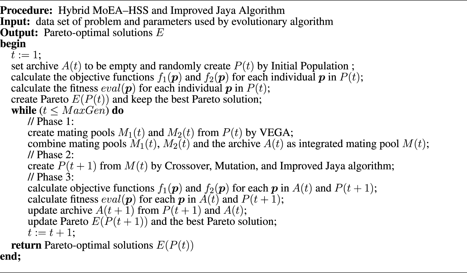
Let n p be a positive constant. Initially, archive is set to empty, and the initial population consists of n ( 0 ) ( ≥ n p ) individuals. For each individual p in population, the objective functions f 1 ( p ) and f 2 ( p ) and the evaluation function e v a l ( p ) are calculated. We adopt the PDDR-FF as the evaluation function e v a l. Let g d ( p ) be the number of individuals that can be dominated by the individual p and g n d ( p ) be the number of individuals that can dominate the individual p. Then,
e v a l p = g d p + 1 g n d p + 1 .
Based on these values, the Pareto-optimal solution in the population is obtained and maintained.
The following three phases are executed in each generation t. In each generation t ( > 1 ), archive A ( t ) contains n a individuals and population P ( t ) contains n ( t ) ( ≥ n p ) individuals generated by genetic operations (Crossover and Mutation) and Improved Jaya algorithm in the previous generation.
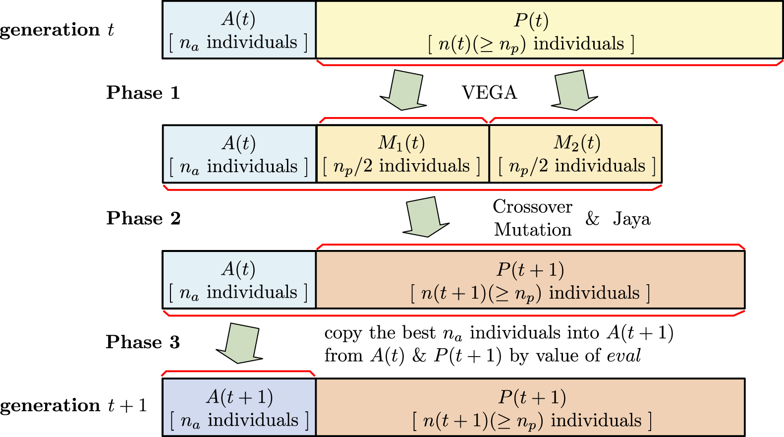
- Phase 1: generating mating pools
- 1. Using the VEGA, two subpopulations M 1 ( t ) and M 2 ( t ), called mating pools from P ( t ), are created. M 1 ( t ) is created by 1 2 n p individuals selected from P ( t ) based only on the value of f 1. Then, the value of f 2 is ignored. Similarly, M 2 ( t ) is created by 1 2 n p individuals selected from P ( t ) based only on the value of f 2.
- 2. An integrated mating pool M ( t ) is created by combining the two mating pools M 1 ( t ) and M 2 ( t ) and Archive A ( t ).
- Phase 2: create P ( t + 1 )
- For individuals in the integrated mating pool M ( t ), Crossover and Mutation operations and the Improved Jaya algorithm are applied, and the t + 1-th generation population P ( t + 1 ) consisting of n p or more individuals is created. These three operations are described in detail in the following.
- Phase 3: create A ( t + 1 )
- 1. For each p in A ( t ) and P ( t + 1 ), the values f 1 ( p ), f 2 ( p ), and e v a l ( p ) are computed.
- 2. A ( t + 1 ) is created by selecting n a individuals from A ( t ) and P ( t + 1 ) in the order of decreasing e v a l value.
Phases 1 – 3 of the proposed method are depicted in Figure 3.
4.2 Chromosome representation and notation
The most natural route expression is adopted as the chromosome expression in the proposed method. For example, if a sequence s: v 0, v 1, v 2, ⋯, v k of vertices is a legal patrolling route, its chromosome representation is a k-tuple p = ( v 0 , v 1 , v 2 , ⋯ , v k − 1 ). The first component of p is considered the starting point. By rotating the genes in p, the chromosome at which the starting point is replaced with v i is denoted by p ( i ). That is,
p i = v i , v i + 1 , ⋯ , v k − 1 , v 0 , v 1 , ⋯ , v i − 1 .
Since GPOPP does not have a fixed starting point, all chromosomes p ( 0 ), p ( 1 ), p ( 2 ), ⋯, p ( k ) represent the same patrolling route. This representation p ( i ) obtained by routing the genes of chromosome p is useful for explaining the genetic operations introduced below. Let V = V be the set of all genes and V p = { v i | 1 ≤ i < k } be the set of genes contained in chromosome p. For each gene v ∈ V, let I v p = { i ∈ I k | v i = v } be the set of gene loci whose gene is v. Let E = E ∪ A and E p = { ⟨ v i , v i + 1 ⟩ | 0 ≤ i < k − 1 } ∪ { ⟨ v k − 1 , v 0 ⟩ } be a set of pairs of adjacent genes in chromosome p and H = H. Genes v k − 1 and v 0 are also considered adjacent. Here, V p = V s and E p = E s. Let v i − and v i + denote the previous and next genes of v i ( 0 ≤ i < k ) in chromosome p, respectively. Here, these gene loci are i − = i − 1 ( mod k ) and i + = i + 1 ( mod k ), where x (mod k) denotes the least nonnegative remainder when x is divided by k. Then, the two sets W u p and W ̄ u p of the gene loci are defined as follows:
- • For each gene u ∈ V p,
W u p = i ∈ I k | v i = u , ⟨ v i − , v i ⟩ , ⟨ v i , v i + ⟩ ∈ E p \ H , ⟨ v i − , v i + ⟩ ∈ E .
- • For each gene u ∉ V p,
W ̄ u p = i ∈ I k | ⟨ v i , v i + ⟩ ∈ E p \ H and ⟨ v i , u ⟩ , ⟨ u , v i + ⟩ ∈ E .
4.3 Initial population
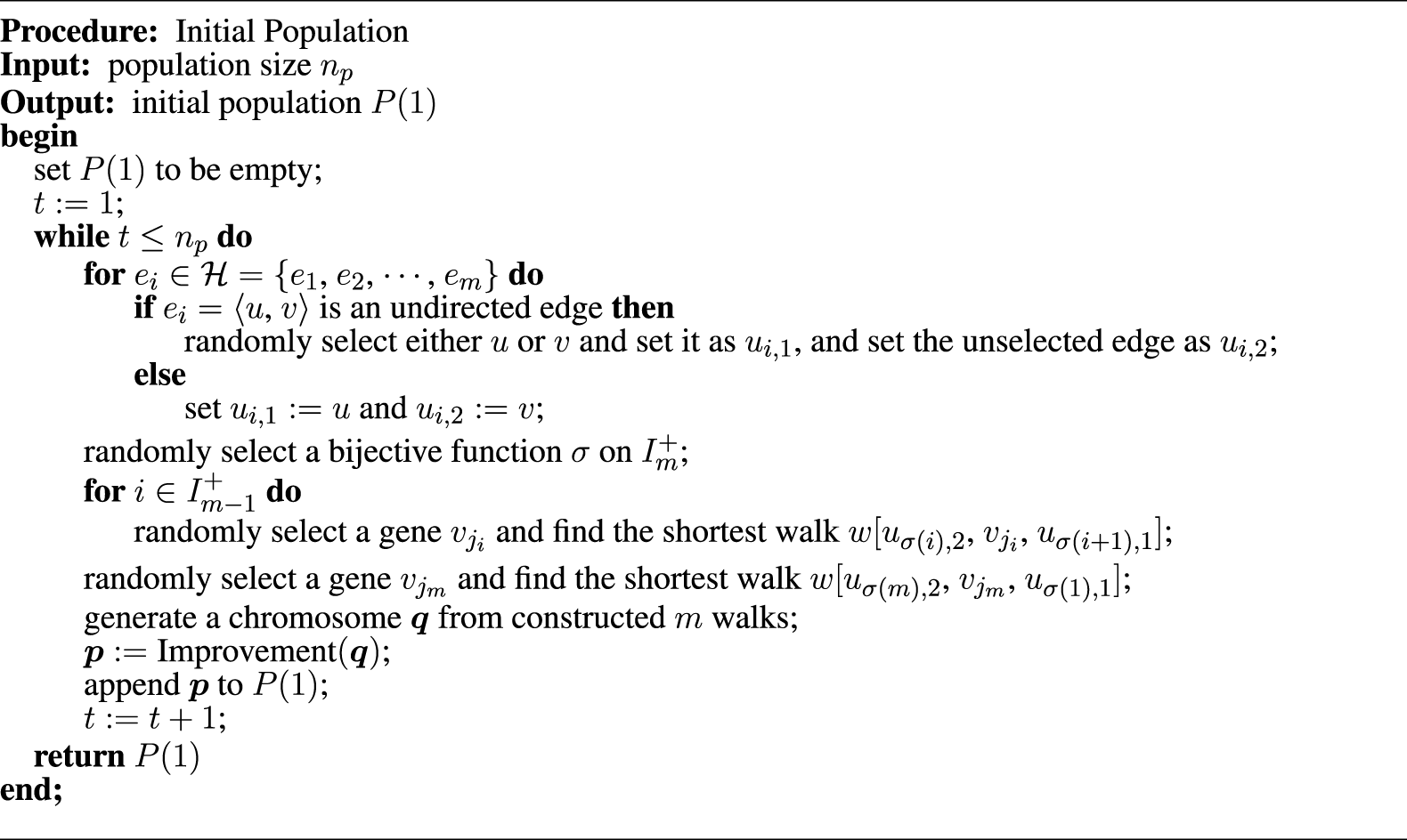
As mentioned in Section 4.1, an initial population consisting of n p individuals is constructed. Each individual in the initial population is generated as follows:
- 1. First, the direction traversing each high-security undirected edge is decided randomly, since because all high-security edges are traversed on every patrolling route.
- 2. Determine the order of traversing high-security edges randomly.
- 3. Generate chromosome q representing the patrolling route that traverses high-security edges in the order determined in step 2. Here, to maintain the diversity of the initial population, two consecutive high-security edges are connected by a shortest path via a randomly selected vertex. The shortest walk w [ u , v , u ′ ] from vertex u to u ′ via v can be determined using the Dijkstra’s algorithm.
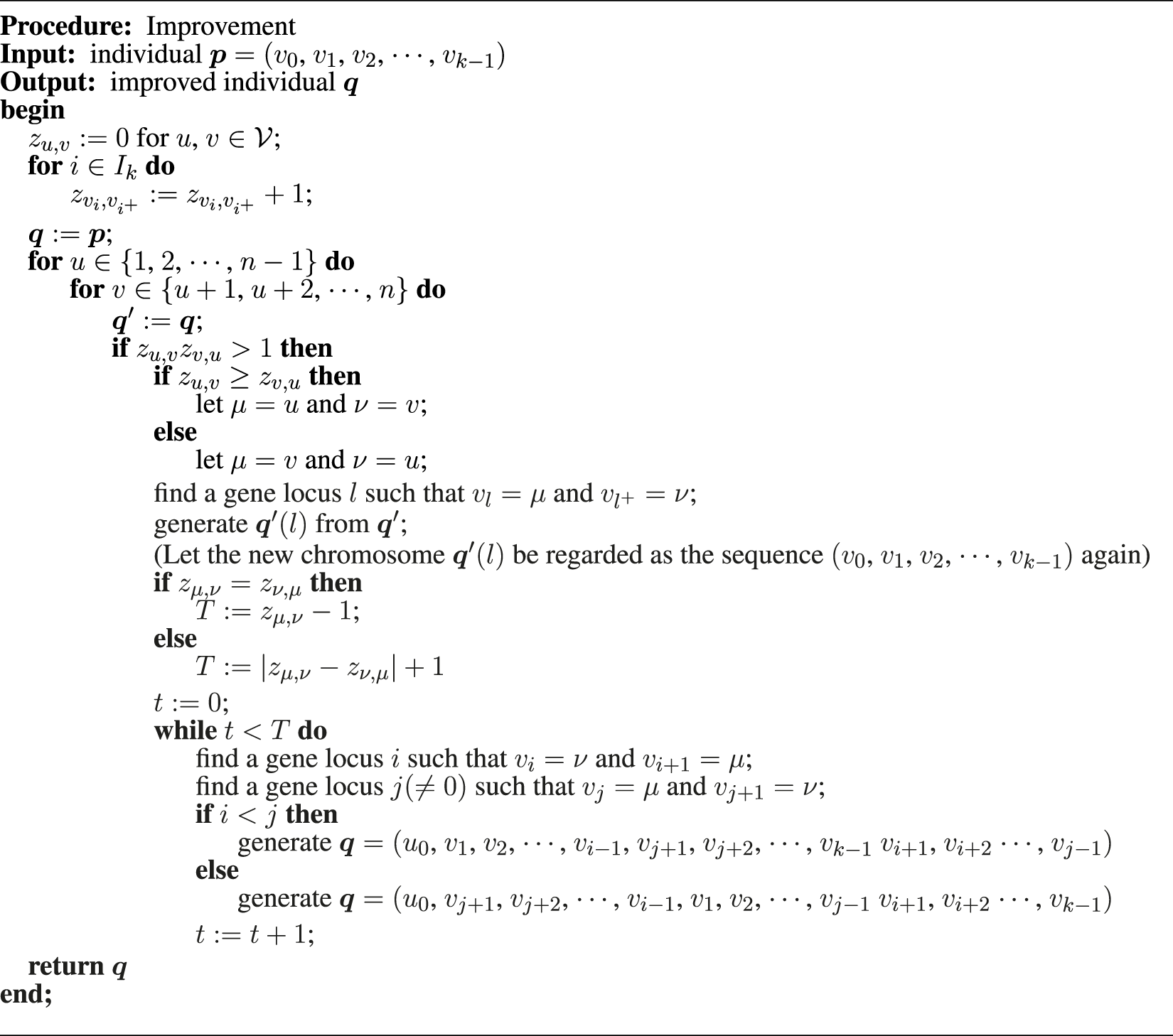
- 4. The patrolling route represented by the generated chromosome q may be able to reduce the total length without changing the noncoverage rate. Therefore, the improvement procedure described below is used for chromosome q generated in step 3.
The pseudocode for the procedure generating the initial population P ( 1 ) consisting of n p individuals is presented in Figure 4.
Let s : v 0, v 1, v 2, ⋯, v k − 1, v k be a patrolling route, and assume that v 0 = v i + 1 = v j = u and v 1 = v i = v j + 1 = v (i, j ∈ I k, i ≠ j). Then, the edge connecting u and v is undirected. If i < j, the edge is traversed three times on s, as shown in the left panel of Figure 5a, and there exists a patrolling route that reduces the total length, as shown in the right panel of Figure 5a. Such a patrolling route traverses all edges on the original route; thus, the noncoverage rate remains unchanged. Similarly, even if j < i, the edge is traversed three times, as shown in the left panel of Figure 5b, and there exists a patrolling route that reduces the total length without changing the noncoverage rate, as shown in the right panel of Figure 5b. In general, assume that undirected edge { u , v } is traversed from u to v l 1 ( ≥ 1 ) times and from v to u l 2 ( ≥ 1 ) times. If l 1 ≠ l 2, there exists a patrolling route that reduces both the number of times traversing from u to v and from v to u by min { l 1 , l 2 } times without changing the noncoverage rate. If l 1 = l 2 > 1, there exists a patrolling route that reduces both the number of times traversing from u to v and from v to u by l 1 − 1 times without changing the noncoverage rate. The pseudocode for the improvement procedure of the chromosome is shown in Figure 6.

4.4 Crossover
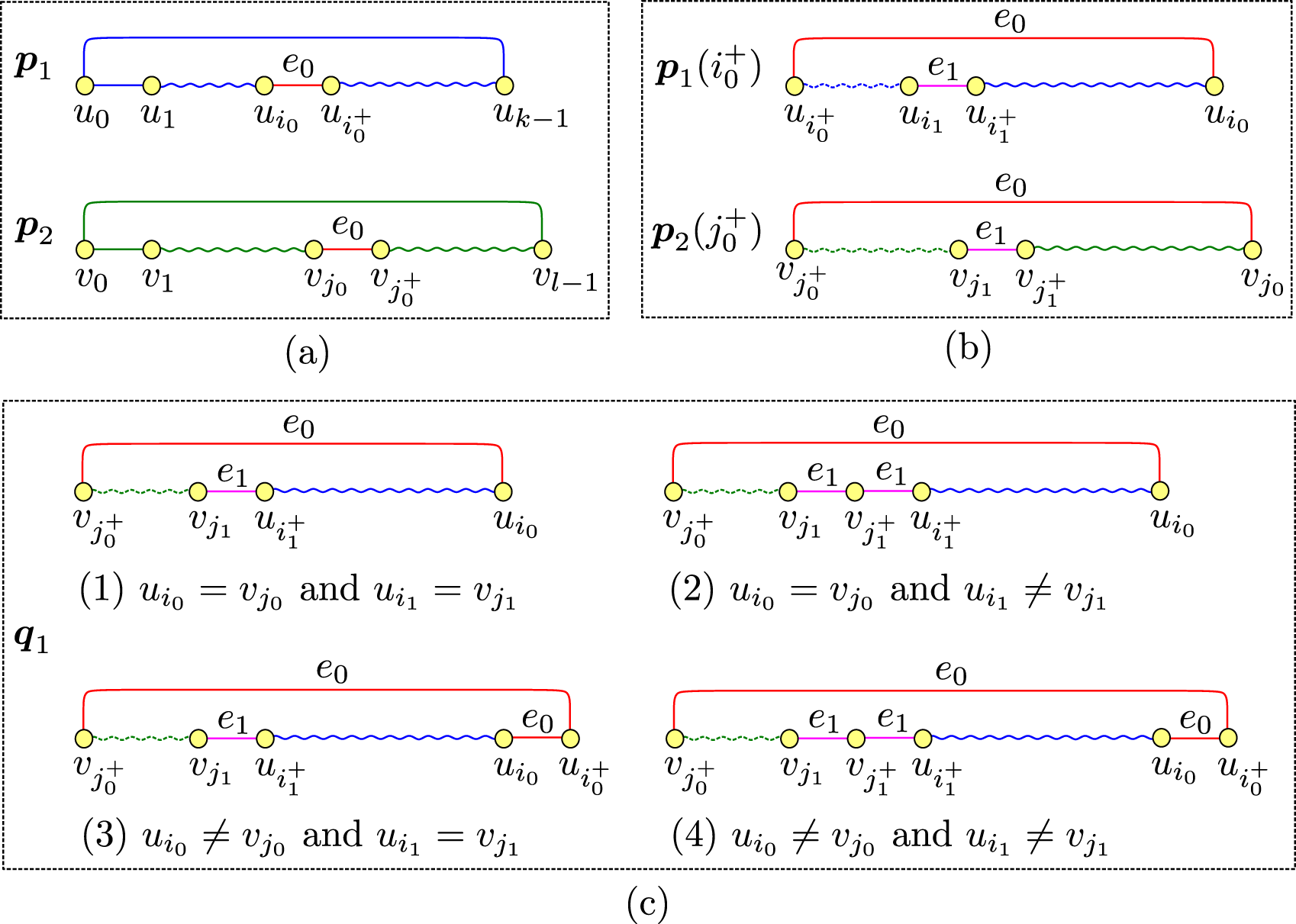
Let p 1 = ( u 0 , u 1 , ⋯ , u k − 1 ) and p 2 = ( v 0 , v 1 , ⋯ , v l − 1 ) be two parent individuals. Then, the crossover operation is used in the proposed method to replace a partial walk on the patrolling route corresponding to p 1 with that corresponding to p 2. The procedure is as follows:
- (a) Any patrolling route requires that all high-security edges are traversed. First, one high-security edge e 0 is randomly selected from H, and one gene u i 0 in p 1 such that e 0 = ⟨ u i 0 , u i 0 + ⟩ and one gene v j 0 in p 2 such that e 0 = ⟨ v j 0 , v j 0 + ⟩ are selected (Figure 7a).
- (b) Find the high-security edge e 1 = ⟨ u i 1 , u i 1 + ⟩ that first appears in the rotated chromosome p 1 ( i 0 + ), and in the rotated chromosome p 2 ( j 0 + ), randomly select one gene v j 1 such that e 1 = ⟨ v j 1 , v j 1 + ⟩ (Figure 7b).
- (c) In the patrolling route corresponding to the chromosome p 1 ( i 0 + ), the partial walk between u i 0 + and u i 1 does not include high-security edges. Therefore, offspring q 1 can be created by replacing this partial walk with the partial walk between v j 0 + and v j 1 in p 2 ( j 0 + ). However, when selected high-security edges e 0 or e 1 are undirected edges, the direction of traversing them on p 1 may differ from the direction of traversing them on p 2. In this case, simply exchanging partial walks does not lead to creating an accurate patrolling route. Based on the direction of traversing e 0 and e 1, the process of creating offspring q 1 can be divided into four steps as follows (Figure 7c): Let q ′ = ( v j 0 + , ⋯ , v j 1 , u i 1 + , ⋯ , u i 0 ) be a chromosome to be created by simply replacing the partial walk from u i 0 + to u i 1 on p 1 ( i 0 + ) with the partial walk v j 0 + to v j 1 on p 2 ( j 0 + ). Then,
- (1) When both e 0 and e 1 are traversed in the same direction on p 1 ( i 0 + ) and p 2 ( j 0 + ) (that is, u i 0 = v j 0 and u i 1 = v j 1), let q 1 ′ be q ′.
- (2) When e 1 is traversed in the opposite direction although e 0 is traversed in the same direction (that is, u i 0 = v j 0 and u i 1 ≠ v j 1), let q 1 ′ be the chromosome created by inserting gene v j 1 + between v j 1 and u i 1 + on q ′.
- (3) When e 0 is traversed in the opposite direction although e 1 is traversed in the same direction (that is, u i 0 ≠ v j 0 and u i 1 = v j 1), let q 1 ′ be the chromosome created by appending gene u i 0 + at the end on q ′.
- (4) When both e 0 and e 1 are traversed in the opposite direction (that is, u i 0 ≠ v j 0 and u i 1 ≠ v j 1), let q 1 ′ be the chromosome created by inserting gene v j 1 + between v j 1 and u i 1 + and by appending gene u i 0 + at the end on q ′.
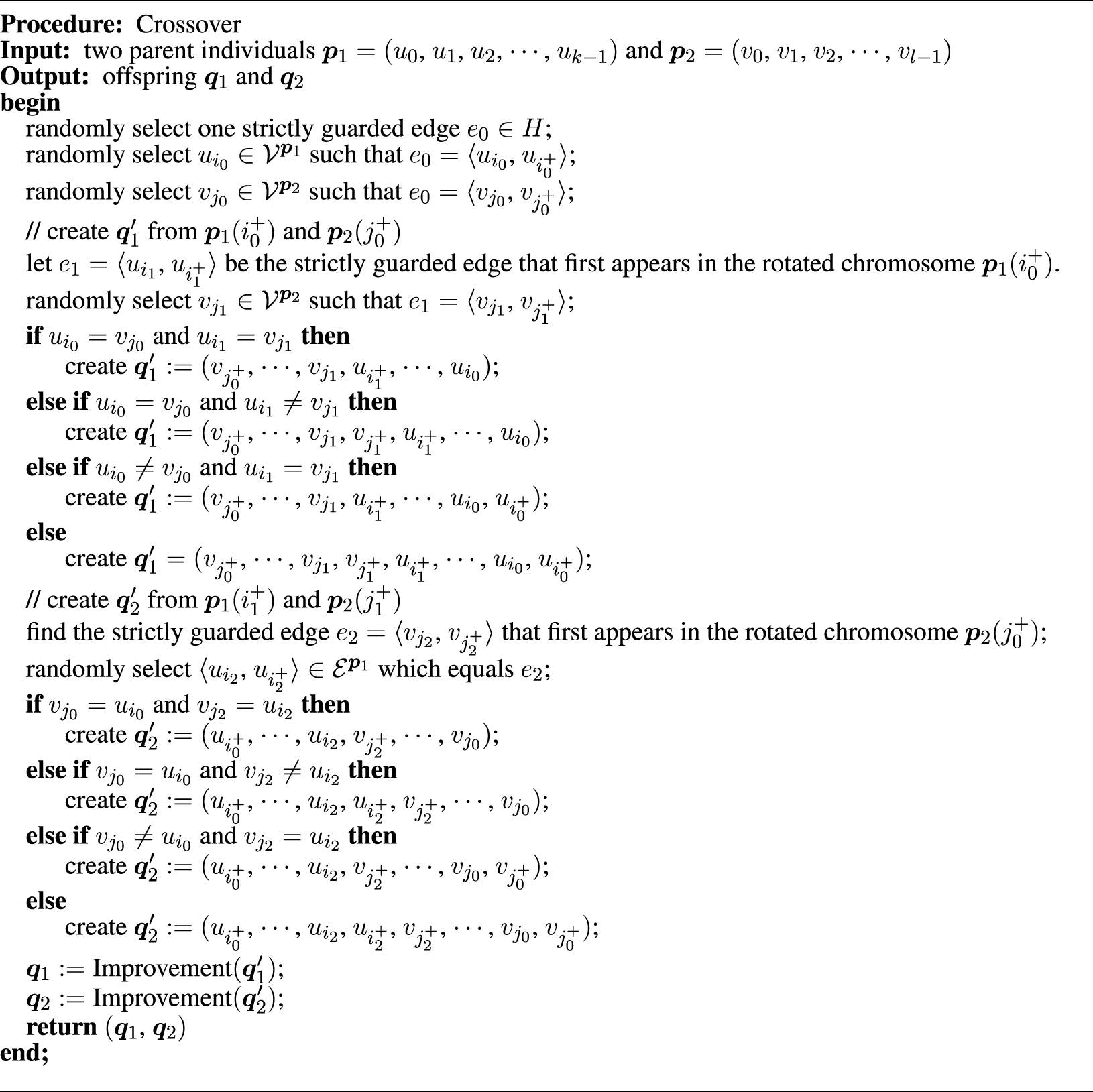
- (d) Find the high-security edge e 2 = ⟨ v j 2 , v j 2 + ⟩ that first appears in the rotated chromosome p 2 ( j 0 + ), and in the rotated chromosome p 1 ( i 0 + ), randomly select one gene u i 2 such that e 2 = ⟨ u i 2 , u i 2 + ⟩. Following the procedure used to create offspring q 1, offspring q 2 ′ is created.
- (e) Create offspring q 1 and q 2 by applying the improvement procedure described in Section 4.3 to q 1 ′ and q 2 ′.
The pseudocode for the proposed crossover operation is presented in Figure 8.
4.5 Mutation
In the crossover operation, the walk of parent individuals tends to be inherited by their offspring. Therefore, it is seldom that generated offspring will traverse vertices or edges that their parents do not. To maintain the diversity of the population, we introduce a mutation operation (Figure 9).
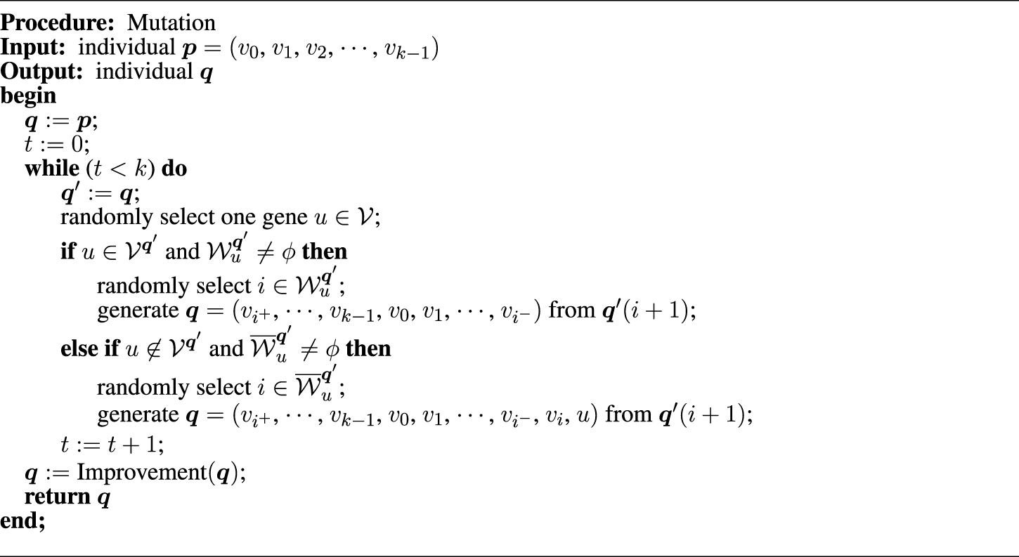
In this operation, the following steps are executed repeatedly: randomly select a gene (vertex) u and
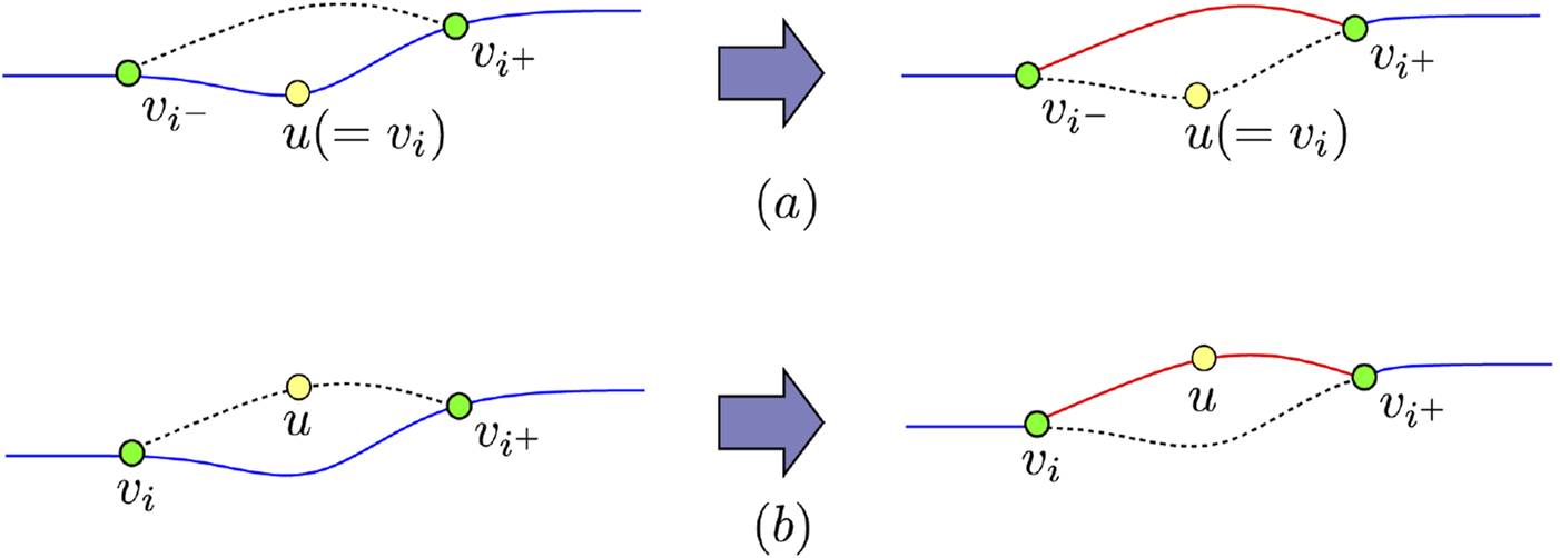
- 1. if gene u exists on the patrolling route corresponding to the chromosome, select one locus i such that v i = u, and if there exists an edge ⟨ v i − , v i + ⟩ connecting vertices v i − and v i + before and after u, remove gene v i from the chromosome (see Figure 10a).
- 2. if gene u does not exist on the patrolling route corresponding to the chromosome and succsessive genes v i and v i + exist on the route such that both ⟨ v i , u ⟩ and ⟨ u , v i + ⟩ are in E, insert gene u between v i and v i + (see Figure 10b).
4.6 Local search strategy based on the Jaya algorithm
The crossover operation introduced in Section 4.4 is an order-based operation in which the orders of traversing the high-security edges of parents and other edges are inherited by offspring. To compensate for the ability to converge the solutions of this crossover, we introduce an improvement strategy that moves dominated solutions closer to a Pareto-optimal solution by combining the strategy used in the mutation operation with the Jaya algorithm.
As mention in Section 2, if the triangle inequality holds, removing a vertex v from the patrolling route tends to reduce the noncovered ratio since edges may be no longer guarded by visual confirmation from v, although the total length of the patrolling route becomes shorter. Conversely, adding a vertex that is not on the patrolling route increases the total length; however, this is expected to improve the noncovered ratio because edges guarded by visual confirmation may increase.
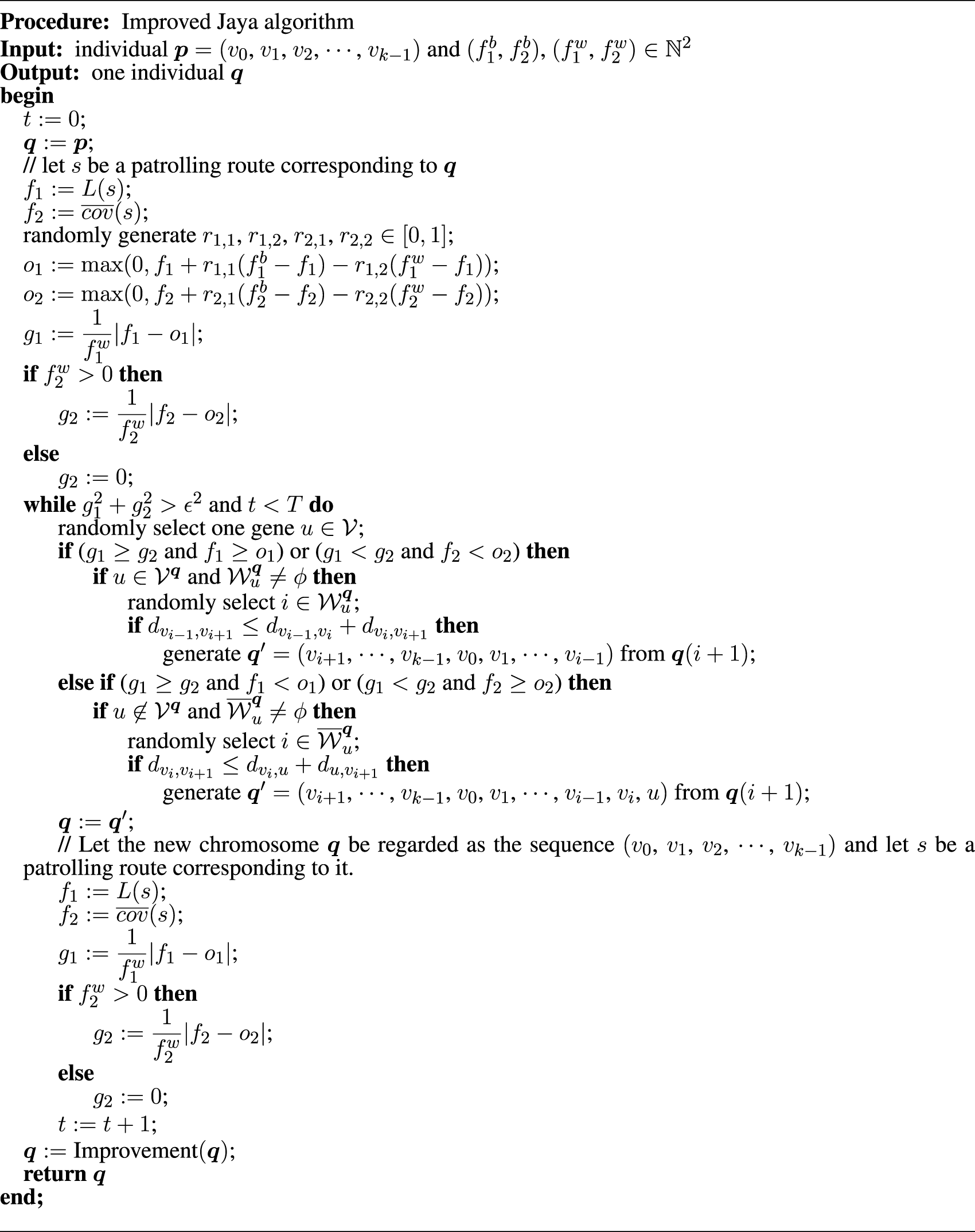
The approach we propose here (called the improved Jaya algorithm below) modifies a given individual to move closer to the best solution and away from the worst solution based on the best and worst candidates in the population. The outline of the proposed strategy is presented in Figure 11. Let p b and p w be the best and worst chromosomes in the current population, respectively, and let s b and s w be the patrolling routes corresponding to p b and p w, respectively. Let ϵ be a sufficiently small positive real number. By putting f 1 b = L ( s b ), f 2 b = c o v ̄ ( s b ), f 1 w = L ( s w ), f 2 w = c o v ̄ ( s w ), the coordinates of s b and s w are ( f 1 b , f 2 b ) and ( f 1 w , f 2 w ), respectively. Then, to modify a certain dominated solution s ( f 1 , f 2 ) to be closer to s b and away from s w, a hypothetical solution s o ( o 1 , o 2 ) is computed based on the strategy of the improved Jaya algorithm. To move s closer to the hypothetical solution s o, the mutation strategy is strategically repeated as follows: Let g 1 = 1 f 1 w | f 1 − o 1 | and g 2 = 1 f 2 w | f 2 − o 2 |, which are normalizations of | f 1 − o 1 | and | f 2 − o 2 |, respectively. If all edges are high-security edges, set g 2 = 0 because f 2 w = 0. The following operations are performed if the triangle inequality holds.
- • if g 1 ≥ g 2, an operation is performed to move the first component of point ( f 1 , f 2 ) closer to the first component of point ( o 1 , o 2 ). Specifically, if f 1 ≥ o 1, vertices are removed from the patrolling route to reduce the total distance; if f 1 < o 1, vertices are added not on the patrolling route increase the total distance.
- • If g 1 < g 2, an operation is performed to move the second component of point ( f 1 , f 2 ) closer to the second component of point ( o 1 , o 2 ). Specifically, if f 2 < o 2, vertices are removed from the patrolling route to reduce the noncovered ratio; if f 2 ≥ o 2, vertices are added not on the patrolling route to increase the noncovered ratio.
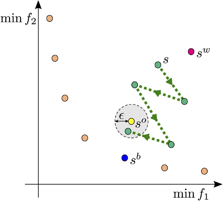
Remark that s o is a hypothetical solution that does not always exist; thus, the operation is repeated until approaching the neighborhood of s o (inside a circle of radius ϵ centered on s o), or the operation is repeated until the terminal condition is reached. The pseudocode for the improved Jaya algorithm is presented in Figure 12.
5 Numerical experiments
In this section, we report the results of numerical experiments conducted to verify the effectiveness of the proposed method (the hybrid strategy of MoEA-HSS and the improved Jaya algorithm) for the GPOPP. In these experiments, we compared the proposed method (called pMH) with the NSGA-II (called NSGA-II) proposed by Deb et al. (2002) and the original MoEA-HSS without the improved Jaya algorithm (called MoEA-HSS). All these methods incorporated the crossover and mutation operations proposed in this paper.
Evaluating the performance of multi-objective optimization methods is not easy since it is difficult to compare the Pareto-optimal solutions (also called the nondominated solutions) obtained by different methods. We compared pMH with NSGA-II and MoEA-HSS using three representative comparison methods. Let N e x be the number of numerical experiments for each method. Let S NSGA - II [ i ], S MoEA - HSS [ i ] and S pMH [ i ] be the Pareto-optimal solution sets of NSGA-II, MoEA-HSS and pMH obtained by the i-th experiment, respectively. The reference solution set S * is defined as the set of nondominated solutions in the union of all Pareto-optimal solution sets ⋃ i ∈ I N e x + S NSGA - II [ i ] ∪ S MoEA - HSS [ i ] ∪ S pMH [ i ].
The three evaluation criteria we used are as follows: where p = 2 and δ x , y = ( f 1 ( y ) − f 1 ( x ) ) 2 + ( f 2 ( y ) − f 2 ( x ) ) 2 denotes the Euclidean distance between a solution x in S α [ i ] and a reference solution y in S *. A smaller G D ( S α [ i ] ) value implies that S α [ i ] is closer to S *. where y ⪯ x means that f ( y ) ≤ f ( x ) holds for any objective function f. The value C ( S α [ i ] , S β [ j ] ) is in the interval [0,1], with values approaching 1 indicating that a greater number of solutions in S β [ j ] are covered by those in S α [ i ].
- 1. Number of nondominated solutions. For each method α ∈{NSGA-II, MoEA-HSS, pMH}, | S α [ i ] | is the number of nondominated solutions obtained by the i-th experiment for α. In general, the selection of the final solution is left to human judgment; thus, the number of Pareto-optimal solutions is an important evaluation criterion.
- 2. Generational distance. For the nondominated solution set S α [ i ] obtained by each method α ∈{NSGA-II, MoEA-HSS, pMH} and the reference solution set S *, the generational distance G D is defined as follows (Van Veldhuizen, 1999; Ishibuchi et al., 2015):
G D S α i = 1 | S α i | ∑ x ∈ S α i min δ x , y | y ∈ S * p 1 p ,
- 3. Coverage of two sets. For two α , β ∈ { NSGA - II , MoEA - HSS , pMH }, where α ≠ β, the coverage C is defined as follows (Zitzler and Thiele, 1999):
C S α i , S β j = x ∈ S β j ∣ ∃ y ∈ S α i , y ⪯ x S β j ,
The benchmark problems used in the experiments were created based on the Mixed Rural Postman Problem (MRPP) benchmark problems RB422 (| V | = 357, | E | = 674, | A | = 210), RB452 (| V | = 465, | E | = 796, | A | = 259), RB472 (| V | = 498, | E | = 849, | A | = 265), RB522 (| V | = 388, | E | = 828, | A | = 278), RB552 (| V | = 488, | E | = 987, | A | = 331) and RB572 (| V | = 498, | E | = 986, | A | = 340) shown in Arc Routing Problems: Data Instances (https://www.uv.es/corberan/instancias.htm). The number of high-security edges (called required edges) defined in the MRPP benchmark problems is sufficiently large. Therefore, they are not suitable for use as benchmarks for methods against the GPOPP in which visual confirmation is allowed. To confirm the effect of visual confirmation, in these experiments, we changed the required edges of each benchmark problem to non-required edges, creating four patterns of benchmark problems with 10, 20, 30, and 40 high-security edges. We used these edges in the experiments. In addition, the ratio of the number of high-security undirected edges to high-security arcs was set to 4 : 1.
The experiments were conducted on a PC with Windows 11, an AMD Ryzen 5 3500 CPU, 3.59 GHz, and 16.0 GB RAM. We conducted preliminary experiments using the benchmark problem RB422_10 with eight high-security undirected edges and two high-security arcs. The parameters were set as follows: the positive constant n p = 150, the archive size n a = 300, the initial population size n ( 0 ) = 300, the crossover rate = 0.3, the mutation rate = 0.05, the terminating condition for the improved Jaya algorithm T = 50, the radius ϵ = 0.1 of a circle centered on the hypothetical solution s o and the maximum generations M a x G e n = 300. When using the improved Jaya algorithm in pMH, the best solution s b is selected from the nondominated solution set S pMH [ i ]. If many nondominated solutions in S pMH [ i ] are concentrated in close proximity, the probability that s b will be selected from among these concentrated individuals increases. Consequently, the individuals generated by the improved Jaya algorithm also tend to move in the direction of the concentrated population. To distribute the location of the individuals generated by the improved Jaya algorithm to some extent, s b was selected as follows: Let m = | S pMH [ i ] | + 10 10 and l = | S pMH [ i ] | ( mod m ). Then
- 1. If m = 1, then let S 1 = S pMH [ i ].
- 2. If m > 1, then partition S pMH [ i ] into m subsets S 1, S 2, ⋯, S m, which satisfy the following conditions:
- • ⋃ i ∈ I m + S i = S pMH [ i ],
- • S i ∩ S j = ϕ (i, j ∈ I m +, i ≠ j),
- • | S i | = | S pMH [ i ] | m (i ∈ I l +), | S j | = | S pMH [ i ] | m (j ∈ I m + \ I l +).
- • For each i ∈ I m − 1 +,
f 1 x < f 1 y ∀ x ∈ S i , ∀ y ∈ ⋃ j ∈ I m + \ I i + S j .
- 3. Randomly select one subset S i from the m subsets, randomly select one solution x from S i, and put s b = x.
We ran 10 numerical experiments for each method (that is, N e x = 10). Comparison results of pMH with NSGA-II and MoEA-HSS at 10, 50, 150 and 300 generations are shown in Table 1. The number of nondominated solutions, generational distance and CPU time are shown in (a) and these are the maximum, minimum, average and standard deviation obtained by 10 experiments. Here, the G D ( S α [ i ] ) for each generation g e n ∈ { 10,50,150,300 } is calculated using the Pareto-optimal solution sets S α [ i ] at the g e n-th generation and the reference solution set S * at the 300th generation. The comparison results for the coverage are shown in (b) and these are calculated by 100 values of C ( S α [ i ] , S β [ j ] ) ( 1 ≤ i , j ≤ N e x ). The evolution of the Pareto-optimal solution set S α [ 1 ] at the 1st experiment for each method is shown in Figure 13.
TABLE 1. Comparison of pMH with NSGA-II and MoEA-HSS during evolution (benchmark problem: RB422_10).
| (a) The number of nondominated solutions, generational distance and CPU time | ||||||||||||
|---|---|---|---|---|---|---|---|---|---|---|---|---|
| Gen | Method | / S α [ i ] / | G D ( S α [ i ] ) | CPU time [sec] | ||||||||
| min | max | ave | std | min | max | ave | std | Ave | ||||
| (b) The coverage of two sets | ||||||||||||
| Gen | Methods | C ( S α [ i ] , S β [ j ] ) | Methods | C ( S α [ i ] , S β [ j ] ) | ||||||||
| α | β | min | max | ave | std | α | β | min | max | ave | std | |
| 10 | NSGA-II | 77 | 117 | 94.0 | 11.06 | 294.56 | 1046.94 | 605.26 | 233.76 | 10.78 | ||
| MoEA-HSS | 75 | 107 | 92.9 | 8.99 | 316.14 | 817.49 | 576.30 | 204.65 | 20.65 | |||
| pMH | 82 | 114 | 98.2 | 9.57 | 160.83 | 679.28 | 410.87 | 161.01 | 51.21 | |||
| 50 | NSGA-II | 176 | 222 | 201.9 | 16.16 | 327.51 | 1073.80 | 569.54 | 197.75 | 58.68 | ||
| MoEA-HSS | 164 | 224 | 197.7 | 16.49 | 362.05 | 756.20 | 520.69 | 135.20 | 107.50 | |||
| pMH | 204 | 269 | 233.2 | 20.83 | 179.55 | 648.16 | 393.76 | 134.40 | 348.96 | |||
| 150 | NSGA-II | 309 | 375 | 328.8 | 22.04 | 59.82 | 267.04 | 141.39 | 64.16 | 148.78 | ||
| MoEA-HSS | 243 | 347 | 307.0 | 26.68 | 46.49 | 251.71 | 122.88 | 71.29 | 276.16 | |||
| pMH | 306 | 431 | 353.4 | 36.27 | 43.48 | 332.89 | 156.66 | 93.84 | 994.56 | |||
| 300 | NSGA-II | 380 | 602 | 471.3 | 69.23 | 9.61 | 141.21 | 51.38 | 38.63 | 264.40 | ||
| MoEA-HSS | 346 | 487 | 396.5 | 34.23 | 17.52 | 193.08 | 76.36 | 46.31 | 518.72 | |||
| pMH | 382 | 603 | 453.3 | 56.59 | 3.17 | 306.90 | 119.06 | 91.86 | 1935.45 | |||
| 10 | pMH | NSGA-II | 0.20 | 1.00 | 0.75 | 0.15 | pMH | MoEA-HSS | 0.17 | 0.98 | 0.65 | 0.17 |
| NSGA-II | pMH | 0.00 | 0.51 | 0.21 | 0.13 | MoEA-HSS | pMH | 0.06 | 0.73 | 0.31 | 0.16 | |
| 50 | pMH | NSGA-II | 0.17 | 1.00 | 0.69 | 0.21 | pMH | MoEA-HSS | 0.23 | 1.00 | 0.68 | 0.19 |
| NSGA-II | pMH | 0.00 | 0.75 | 0.25 | 0.18 | MoEA-HSS | pMH | 0.00 | 0.67 | 0.26 | 0.17 | |
| 150 | pMH | NSGA-II | 0.17 | 1.00 | 0.65 | 0.22 | pMH | MoEA-HSS | 0.14 | 1.00 | 0.61 | 0.23 |
| NSGA-II | pMH | 0.00 | 0.78 | 0.33 | 0.22 | MoEA-HSS | pMH | 0.00 | 0.88 | 0.34 | 0.22 | |
| 300 | pMH | NSGA-II | 0.02 | 1.00 | 0.59 | 0.26 | pMH | MoEA-HSS | 0.02 | 1.00 | 0.58 | 0.28 |
| NSGA-II | pMH | 0.00 | 0.95 | 0.38 | 0.25 | MoEA-HSS | pMH | 0.00 | 0.92 | 0.39 | 0.27 |
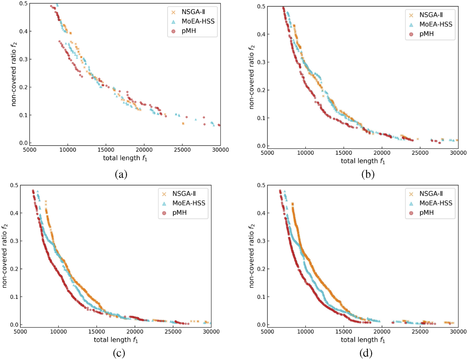
The number of nondominated solutions | S α [ i ] | for NSGA-II and pMH are no significant difference, although the value for MoEA-HSS is slightly lower. If the Pareto-optimal solution set S α [ i ] contains even a single solution that is far from S *, the generational distance will have a large value. Therefore, method α cannot be considered inferior simply because the generational distance has a large value. On the other hand, when the minimum value of the generational distance is sufficiently small, method α is considered superior because the nondominated solutions obtained by method α are likely to be close to the solutions in the reference solution set S *. For these reasons, it is more appropriate to use the minimum value, rather than the average or maximum, when conducting evaluations with the generational distance. Therefore, from these experimental results, in evaluations based on the number of nondominated solutions and the generational distance, pMH can be considered superior to other methods. In particular, the comparison between MoEA-HSS and pMH based on these criteria implies that the ability of local search for the improved Jaya algorithm has achieved the expected results.
The coverage C ( S α [ i ] , S β [ j ] ) is the rate that solutions in S β [ j ] are covered by solutions in S α [ i ]. Hence, if the average of C ( S α [ i ] , S β [ j ] ) is higher than the average of C ( S β [ j ] , S α [ i ] ), S α [ i ] can be considered as better than S β [ i ] under this criterion. Therefore, by comparing the average of two coverages C ( S pMH [ i ] , S β [ j ] ) and C ( S β [ j ] , S pMH [ i ] ) (β ∈{NSGA-II, MoEA-HSS}), the Pareto-optimal solution set S pMH [ i ] is considered statistically superior to S β [ j ] obtained by other methods at every generations.
The experiment results of comparing pMH with NSGA-II and MoEA-HSS when we ran each method until 300 generations for all benchmark problems are shown in Tables 2, 3.
TABLE 2. Comparison of pMH with NSGA-II and MoEA-HSS by the number of nondominated solutions, generational distance and CPU time ( gen = 300 ).
| Problem | Method | / S α [ i ] / | G D ( S α [ i ] ) | CPU time [sec] | ||||||
|---|---|---|---|---|---|---|---|---|---|---|
| min | max | ave | std | min | max | ave | std | Ave | ||
| RB422_10 | NSGA-II | 380 | 602 | 471.3 | 69.23 | 9.61 | 141.21 | 51.38 | 38.63 | 264.40 |
| MoEA-HSS | 346 | 487 | 396.5 | 34.23 | 17.52 | 193.08 | 76.36 | 46.31 | 518.72 | |
| pMH | 382 | 603 | 453.3 | 56.59 | 3.17 | 306.90 | 119.06 | 91.86 | 1935.45 | |
| RB422_20 | NSGA-II | 262 | 481 | 369.4 | 59.40 | 5.61 | 162.38 | 74.24 | 53.30 | 375.92 |
| MoEA-HSS | 264 | 421 | 324.7 | 43.54 | 5.26 | 199.14 | 100.44 | 68.67 | 651.91 | |
| pMH | 254 | 414 | 357.1 | 50.74 | 2.48 | 212.85 | 123.89 | 60.97 | 2036.05 | |
| RB422_30 | NSGA-II | 152 | 323 | 214.0 | 48.24 | 41.17 | 239.79 | 132.88 | 56.13 | 489.67 |
| MoEA-HSS | 145 | 264 | 208.4 | 32.63 | 54.19 | 274.29 | 119.93 | 67.00 | 767.79 | |
| pMH | 193 | 301 | 236.5 | 38.91 | 34.76 | 313.97 | 165.31 | 89.84 | 2340.67 | |
| RB422_40 | NSGA-II | 129 | 390 | 207.0 | 76.84 | 18.56 | 125.78 | 65.43 | 35.55 | 626.15 |
| MoEA-HSS | 113 | 245 | 175.5 | 35.93 | 15.12 | 134.20 | 76.34 | 39.70 | 1021.97 | |
| pMH | 168 | 271 | 210.4 | 30.58 | 11.13 | 301.42 | 90.95 | 79.47 | 2609.41 | |
| RB452_10 | NSGA-II | 409 | 580 | 481.6 | 48.96 | 7.12 | 28.18 | 19.44 | 7.78 | 459.99 |
| MoEA-HSS | 345 | 429 | 398.2 | 25.21 | 8.84 | 64.65 | 29.00 | 19.70 | 828.12 | |
| pMH | 423 | 506 | 454.6 | 28.84 | 6.69 | 165.06 | 58.78 | 52.18 | 3095.65 | |
| RB452_20 | NSGA-II | 269 | 412 | 338.4 | 49.93 | 17.39 | 254.83 | 64.91 | 69.65 | 678.07 |
| MoEA-HSS | 226 | 332 | 272.1 | 32.53 | 15.65 | 510.43 | 154.60 | 154.38 | 1255.28 | |
| pMH | 268 | 441 | 352.9 | 46.15 | 12.06 | 546.01 | 186.63 | 180.61 | 3855.40 | |
| RB452_30 | NSGA-II | 158 | 330 | 237.1 | 54.69 | 24.62 | 233.80 | 127.72 | 68.65 | 889.09 |
| MoEA-HSS | 186 | 283 | 227.5 | 28.82 | 26.47 | 412.35 | 172.84 | 110.71 | 1471.48 | |
| pMH | 245 | 380 | 298.5 | 39.55 | 22.86 | 559.41 | 243.63 | 166.04 | 4346.86 | |
| RB452_40 | NSGA-II | 129 | 238 | 175.1 | 31.41 | 60.63 | 436.12 | 255.00 | 115.72 | 1099.45 |
| MoEA-HSS | 126 | 233 | 163.9 | 31.97 | 65.13 | 507.44 | 227.02 | 145.80 | 1748.62 | |
| pMH | 172 | 264 | 222.8 | 33.74 | 52.26 | 248.59 | 155.26 | 58.32 | 5117.44 | |
| RB472_10 | NSGA-II | 525 | 685 | 604.1 | 55.70 | 7.11 | 150.77 | 38.78 | 42.20 | 593.61 |
| MoEA-HSS | 405 | 508 | 463.1 | 36.36 | 18.50 | 204.54 | 73.27 | 64.95 | 904.46 | |
| pMH | 421 | 597 | 497.1 | 44.95 | 4.85 | 175.62 | 43.97 | 51.60 | 2850.32 | |
| RB472_20 | NSGA-II | 322 | 423 | 370.6 | 30.89 | 85.91 | 838.67 | 307.09 | 234.65 | 1114.77 |
| MoEA-HSS | 275 | 426 | 329.6 | 43.93 | 93.13 | 556.72 | 240.50 | 129.08 | 1795.23 | |
| pMH | 281 | 399 | 341.0 | 39.31 | 13.98 | 440.36 | 156.16 | 122.68 | 3966.87 | |
| RB472_30 | NSGA-II | 196 | 374 | 274.2 | 46.82 | 77.76 | 706.68 | 400.50 | 182.09 | 1486.01 |
| MoEA-HSS | 168 | 321 | 245.3 | 44.29 | 141.41 | 913.16 | 365.27 | 227.03 | 2419.09 | |
| pMH | 180 | 294 | 259.1 | 34.15 | 12.81 | 435.61 | 175.33 | 123.11 | 4964.62 | |
| RB472_40 | NSGA-II | 99 | 272 | 180.4 | 45.17 | 263.60 | 1072.71 | 586.71 | 258.87 | 1888.19 |
| MoEA-HSS | 161 | 242 | 187.8 | 28.20 | 164.50 | 912.41 | 420.79 | 199.80 | 3115.36 | |
| pMH | 110 | 262 | 184.7 | 53.48 | 29.16 | 524.68 | 242.39 | 151.61 | 6235.13 | |
| RB522_10 | NSGA-II | 528 | 633 | 562.4 | 36.67 | 4.05 | 67.74 | 25.74 | 20.94 | 298.48 |
| MoEA-HSS | 393 | 486 | 441.2 | 32.17 | 5.23 | 192.04 | 47.89 | 51.94 | 589.38 | |
| pMH | 428 | 575 | 492.4 | 38.31 | 1.43 | 109.03 | 34.00 | 32.35 | 2422.35 | |
| RB522_20 | NSGA-II | 283 | 423 | 357.5 | 35.05 | 24.87 | 50.94 | 35.25 | 9.45 | 412.07 |
| MoEA-HSS | 201 | 331 | 261.2 | 45.00 | 10.65 | 105.69 | 40.91 | 32.72 | 511.92 | |
| pMH | 244 | 373 | 311.3 | 43.49 | 3.45 | 66.84 | 28.43 | 18.13 | 2345.58 | |
| RB522_30 | NSGA-II | 155 | 336 | 250.2 | 58.69 | 15.76 | 164.57 | 74.84 | 45.32 | 507.85 |
| MoEA-HSS | 179 | 298 | 243.8 | 39.74 | 14.20 | 103.95 | 59.66 | 30.82 | 639.69 | |
| pMH | 126 | 270 | 193.5 | 38.71 | 1.80 | 211.54 | 75.44 | 65.55 | 3419.29 | |
| RB522_40 | NSGA-II | 132 | 300 | 209.9 | 52.08 | 94.27 | 308.58 | 158.19 | 61.62 | 629.45 |
| MoEA-HSS | 110 | 196 | 160.6 | 26.50 | 21.78 | 214.40 | 121.46 | 49.36 | 729.41 | |
| pMH | 110 | 248 | 181.4 | 38.93 | 0.89 | 229.42 | 134.67 | 68.10 | 2994.47 | |
| RB552_10 | NSGA-II | 441 | 578 | 520.7 | 46.44 | 12.03 | 66.23 | 36.23 | 21.71 | 363.79 |
| MoEA-HSS | 362 | 464 | 435.4 | 28.95 | 14.06 | 130.60 | 42.45 | 38.14 | 634.52 | |
| pMH | 417 | 522 | 475.4 | 30.80 | 11.98 | 195.67 | 49.70 | 51.69 | 4273.26 | |
| RB552_20 | NSGA-II | 269 | 406 | 324.9 | 41.96 | 12.63 | 288.89 | 69.49 | 76.71 | 493.70 |
| MoEA-HSS | 251 | 344 | 307.2 | 27.99 | 12.84 | 243.47 | 111.28 | 68.44 | 982.66 | |
| pMH | 330 | 408 | 368.6 | 27.92 | 12.17 | 462.37 | 174.80 | 128.41 | 5186.40 | |
| RB552_30 | NSGA-II | 190 | 334 | 272.2 | 44.52 | 27.32 | 226.11 | 124.58 | 61.44 | 606.83 |
| MoEA-HSS | 153 | 308 | 212.9 | 51.19 | 30.41 | 234.74 | 152.43 | 57.37 | 984.32 | |
| pMH | 249 | 375 | 303.8 | 32.03 | 18.59 | 493.17 | 207.32 | 141.31 | 5069.98 | |
| RB552_40 | NSGA-II | 124 | 229 | 184.2 | 33.68 | 39.87 | 460.09 | 133.89 | 114.07 | 939.13 |
| MoEA-HSS | 135 | 273 | 187.1 | 40.84 | 25.67 | 296.67 | 125.01 | 92.27 | 1153.40 | |
| pMH | 188 | 327 | 250.2 | 38.14 | 20.82 | 244.69 | 118.60 | 66.34 | 5472.13 | |
| RB572_10 | NSGA-II | 428 | 589 | 520.1 | 48.10 | 18.18 | 76.48 | 39.99 | 17.82 | 478.17 |
| MoEA-HSS | 372 | 475 | 416.1 | 29.46 | 3.34 | 431.67 | 93.25 | 119.77 | 622.80 | |
| pMH | 406 | 499 | 445.6 | 28.46 | 2.09 | 156.54 | 63.03 | 48.49 | 3710.57 | |
| RB572_20 | NSGA-II | 281 | 402 | 334.7 | 32.96 | 16.98 | 139.31 | 51.33 | 34.76 | 536.94 |
| MoEA-HSS | 231 | 334 | 285.5 | 29.64 | 9.57 | 268.10 | 67.75 | 75.43 | 825.95 | |
| pMH | 290 | 374 | 344.5 | 24.74 | 7.92 | 115.86 | 53.32 | 34.91 | 4368.54 | |
| RB572_30 | NSGA-II | 163 | 254 | 212.7 | 25.97 | 26.61 | 222.26 | 93.67 | 53.94 | 600.63 |
| MoEA-HSS | 156 | 260 | 218.6 | 30.93 | 19.42 | 85.66 | 53.82 | 21.80 | 1356.75 | |
| pMH | 244 | 346 | 284.5 | 33.21 | 3.48 | 140.03 | 60.36 | 35.76 | 5328.90 | |
| RB572_40 | NSGA-II | 146 | 255 | 177.9 | 29.71 | 9.18 | 273.45 | 103.84 | 77.19 | 715.96 |
| MoEA-HSS | 149 | 231 | 190.9 | 28.41 | 11.64 | 452.21 | 91.76 | 122.21 | 1610.60 | |
| pMH | 180 | 302 | 243.0 | 36.25 | 6.15 | 222.99 | 83.88 | 59.41 | 5029.07 |
TABLE 3. Comparison of pMH with NSGA-II and MoEA-HSS by the coverage ( gen = 300 ).
| Problem | Methods | C ( S α [ i ] , S β [ j ] ) | Methods | C ( S α [ i ] , S β [ j ] ) | ||||||||
|---|---|---|---|---|---|---|---|---|---|---|---|---|
| α | β | min | max | ave | std | α | β | min | max | ave | std | |
| RB422_10 | pMH | NSGA-II | 0.02 | 1.00 | 0.59 | 0.26 | pMH | MoEA-HSS | 0.02 | 1.00 | 0.58 | 0.28 |
| NSGA-II | pMH | 0.00 | 0.95 | 0.38 | 0.25 | MoEA-HSS | pMH | 0.00 | 0.92 | 0.39 | 0.27 | |
| RB422_20 | pMH | NSGA-II | 0.00 | 1.00 | 0.66 | 0.28 | pMH | MoEA-HSS | 0.00 | 0.97 | 0.57 | 0.29 |
| NSGA-II | pMH | 0.00 | 0.98 | 0.31 | 0.28 | MoEA-HSS | pMH | 0.01 | 1.00 | 0.40 | 0.28 | |
| RB422_30 | pMH | NSGA-II | 0.00 | 1.00 | 0.65 | 0.31 | pMH | MoEA-HSS | 0.00 | 1.00 | 0.47 | 0.34 |
| NSGA-II | pMH | 0.00 | 1.00 | 0.30 | 0.29 | MoEA-HSS | pMH | 0.01 | 1.00 | 0.47 | 0.34 | |
| RB422_40 | pMH | NSGA-II | 0.00 | 1.00 | 0.73 | 0.29 | pMH | MoEA-HSS | 0.00 | 1.00 | 0.61 | 0.29 |
| NSGA-II | pMH | 0.00 | 0.99 | 0.20 | 0.25 | MoEA-HSS | pMH | 0.00 | 0.98 | 0.27 | 0.26 | |
| RB452_10 | pMH | NSGA-II | 0.06 | 1.00 | 0.63 | 0.21 | pMH | MoEA-HSS | 0.00 | 1.00 | 0.52 | 0.28 |
| NSGA-II | pMH | 0.00 | 0.83 | 0.32 | 0.21 | MoEA-HSS | pMH | 0.00 | 1.00 | 0.41 | 0.27 | |
| RB452_20 | pMH | NSGA-II | 0.00 | 0.98 | 0.49 | 0.29 | pMH | MoEA-HSS | 0.00 | 0.96 | 0.38 | 0.30 |
| NSGA-II | pMH | 0.00 | 1.00 | 0.44 | 0.30 | MoEA-HSS | pMH | 0.03 | 1.00 | 0.54 | 0.31 | |
| RB452_30 | pMH | NSGA-II | 0.00 | 1.00 | 0.44 | 0.37 | pMH | MoEA-HSS | 0.00 | 1.00 | 0.40 | 0.37 |
| NSGA-II | pMH | 0.00 | 1.00 | 0.50 | 0.36 | MoEA-HSS | pMH | 0.00 | 1.00 | 0.55 | 0.37 | |
| RB452_40 | pMH | NSGA-II | 0.00 | 1.00 | 0.59 | 0.36 | pMH | MoEA-HSS | 0.00 | 1.00 | 0.49 | 0.38 |
| NSGA-II | pMH | 0.00 | 1.00 | 0.34 | 0.34 | MoEA-HSS | pMH | 0.00 | 1.00 | 0.40 | 0.35 | |
| RB472_10 | pMH | NSGA-II | 0.19 | 1.00 | 0.61 | 0.24 | pMH | MoEA-HSS | 0.01 | 1.00 | 0.65 | 0.28 |
| NSGA-II | pMH | 0.00 | 0.71 | 0.31 | 0.21 | MoEA-HSS | pMH | 0.00 | 0.92 | 0.30 | 0.27 | |
| RB472_20 | pMH | NSGA-II | 0.00 | 1.00 | 0.78 | 0.31 | pMH | MoEA-HSS | 0.02 | 1.00 | 0.65 | 0.36 |
| NSGA-II | pMH | 0.00 | 1.00 | 0.20 | 0.31 | MoEA-HSS | pMH | 0.00 | 0.98 | 0.31 | 0.35 | |
| RB472_30 | pMH | NSGA-II | 0.00 | 1.00 | 0.78 | 0.29 | pMH | MoEA-HSS | 0.02 | 1.00 | 0.83 | 0.25 |
| NSGA-II | pMH | 0.00 | 1.00 | 0.19 | 0.27 | MoEA-HSS | pMH | 0.00 | 0.92 | 0.12 | 0.21 | |
| RB472_40 | pMH | NSGA-II | 0.05 | 1.00 | 0.78 | 0.32 | pMH | MoEA-HSS | 0.01 | 1.00 | 0.65 | 0.36 |
| NSGA-II | pMH | 0.00 | 0.98 | 0.17 | 0.28 | MoEA-HSS | pMH | 0.00 | 0.99 | 0.30 | 0.34 | |
| RB522_10 | pMH | NSGA-II | 0.00 | 0.94 | 0.44 | 0.22 | pMH | MoEA-HSS | 0.04 | 1.00 | 0.53 | 0.28 |
| NSGA-II | pMH | 0.02 | 1.00 | 0.47 | 0.24 | MoEA-HSS | pMH | 0.00 | 0.96 | 0.44 | 0.27 | |
| RB522_20 | pMH | NSGA-II | 0.00 | 1.00 | 0.59 | 0.28 | pMH | MoEA-HSS | 0.00 | 1.00 | 0.46 | 0.31 |
| NSGA-II | pMH | 0.00 | 0.98 | 0.37 | 0.29 | MoEA-HSS | pMH | 0.00 | 1.00 | 0.50 | 0.32 | |
| RB522_30 | pMH | NSGA-II | 0.00 | 1.00 | 0.67 | 0.33 | pMH | MoEA-HSS | 0.00 | 1.00 | 0.77 | 0.28 |
| NSGA-II | pMH | 0.00 | 1.00 | 0.27 | 0.29 | MoEA-HSS | pMH | 0.00 | 1.00 | 0.18 | 0.26 | |
| RB522_40 | pMH | NSGA-II | 0.00 | 1.00 | 0.65 | 0.37 | pMH | MoEA-HSS | 0.00 | 1.00 | 0.53 | 0.40 |
| NSGA-II | pMH | 0.00 | 0.99 | 0.31 | 0.36 | MoEA-HSS | pMH | 0.00 | 1.00 | 0.43 | 0.40 | |
| RB552_10 | pMH | NSGA-II | 0.21 | 1.00 | 0.66 | 0.17 | pMH | MoEA-HSS | 0.02 | 0.95 | 0.56 | 0.26 |
| NSGA-II | pMH | 0.00 | 0.68 | 0.29 | 0.17 | MoEA-HSS | pMH | 0.02 | 0.98 | 0.38 | 0.25 | |
| RB552_20 | pMH | NSGA-II | 0.01 | 1.00 | 0.79 | 0.20 | pMH | MoEA-HSS | 0.01 | 0.99 | 0.66 | 0.26 |
| NSGA-II | pMH | 0.00 | 0.90 | 0.19 | 0.20 | MoEA-HSS | pMH | 0.01 | 0.99 | 0.30 | 0.24 | |
| RB552_30 | pMH | NSGA-II | 0.00 | 0.99 | 0.62 | 0.29 | pMH | MoEA-HSS | 0.00 | 1.00 | 0.44 | 0.28 |
| NSGA-II | pMH | 0.00 | 1.00 | 0.32 | 0.26 | MoEA-HSS | pMH | 0.01 | 1.00 | 0.42 | 0.24 | |
| RB552_40 | pMH | NSGA-II | 0.00 | 1.00 | 0.61 | 0.29 | pMH | MoEA-HSS | 0.00 | 1.00 | 0.59 | 0.32 |
| NSGA-II | pMH | 0.00 | 0.98 | 0.30 | 0.26 | MoEA-HSS | pMH | 0.00 | 1.00 | 0.31 | 0.31 | |
| RB572_10 | pMH | NSGA-II | 0.09 | 1.00 | 0.52 | 0.22 | pMH | MoEA-HSS | 0.02 | 0.98 | 0.55 | 0.26 |
| NSGA-II | pMH | 0.00 | 0.86 | 0.42 | 0.23 | MoEA-HSS | pMH | 0.02 | 0.95 | 0.41 | 0.24 | |
| RB572_20 | pMH | NSGA-II | 0.05 | 0.99 | 0.64 | 0.29 | pMH | MoEA-HSS | 0.00 | 0.97 | 0.39 | 0.29 |
| NSGA-II | pMH | 0.00 | 0.96 | 0.34 | 0.29 | MoEA-HSS | pMH | 0.01 | 0.97 | 0.55 | 0.29 | |
| RB572_30 | pMH | NSGA-II | 0.00 | 1.00 | 0.62 | 0.26 | pMH | MoEA-HSS | 0.02 | 1.00 | 0.57 | 0.27 |
| NSGA-II | pMH | 0.00 | 0.91 | 0.31 | 0.23 | MoEA-HSS | pMH | 0.00 | 0.95 | 0.36 | 0.25 | |
| RB572_40 | pMH | NSGA-II | 0.02 | 1.00 | 0.74 | 0.25 | pMH | MoEA-HSS | 0.00 | 0.98 | 0.60 | 0.24 |
| NSGA-II | pMH | 0.00 | 0.97 | 0.20 | 0.23 | MoEA-HSS | pMH | 0.00 | 1.00 | 0.31 | 0.23 |
Our method pMH achieved better results than other methods in all benchmark problems with respect to the generational distance and the coverage of two sets, although pMH and NSGA-II are evenly-matched at the criterion the number of nondominated solutions. Here, even if pMH is inferior to that of other methods α at the criteria the number of nondominated solutions, since it is considered that the ratio of solutions in S α [ j ] covered by solutions in S pMH [ i ] is high, S pMH [ i ] is not necessarily inferior to S NSGA - II [ j ] or S MoEA - HSS [ j ]. Based on these numerical experiments, we confirmed that the local search based on the improved Jaya algorithm is effective and that pMH can generate superior Pareto-optimal solutions.
6 Conclusion
In this study, we defined a new arc routing bi-objective optimization problem (GPOPP) that models the patrol security of police officers (or security guards) based on the POPP and proposed a hybrid heuristic approach for the GPOPP. The proposed method combines the hybrid sampling strategy MoEA-HSS, which combines sampling strategies based on the VEGA and PDDR-FF, with a solution improvement strategy based on the improved Jaya algorithm. The solutions of the MoEA-HSS approach to the true Pareto differ in various directions because the VEGA-based sampling strategy has a preference for the edge region of the Pareto front and the PDDR-FF-based sampling strategy tends to converge toward the center area of the Pareto front. The proposed method (pMH) improves convergence by combining the MoEA-HSS with the improved Jaya algorithm-based local search method. The numerical experimental results demonstrate that the proposed method can obtain better solutions than the NSGA-II and the MoEA-HSS. The remaining challenge for us is to improve efficiency by reducing CPU time while maintaining high solution quality. In addition, extending GPOPP model will enable us to more accurately replicate the complex challenges of real-world urban policing. One extension would be to model situations where multiple officers work together, and we consider to adapt our method to address such extended problems.
Generative AI statement
The author(s) declare that no Generative AI was used in the creation of this manuscript.
Publisher’s note
All claims expressed in this article are solely those of the authors and do not necessarily represent those of their affiliated organizations, or those of the publisher, the editors and the reviewers. Any product that may be evaluated in this article, or claim that may be made by its manufacturer, is not guaranteed or endorsed by the publisher.
Statements
- Conflict of interest
The authors declare that the research was conducted in the absence of any commercial or financial relationships that could be construed as a potential conflict of interest.
- Funding
The author(s) declare that financial support was received for the research and/or publication of this article. This work was supported by research funding provided by the Maebashi Institute of Technology, Japan.
- Data availability
The raw data supporting the conclusions of this article will be made available by the authors, without undue reservation.
- Author contributions
FK: Writing – review and editing, Writing – original draft. HT: Writing – original draft, Writing – review and editing. MT: Writing – original draft, Writing – review and editing.
References
- Aiello G., La Scalia G., Enea M. (2012). A multi objective genetic algorithm for the facility layout problem based upon slicing structure encoding. Expert Syst. Appl. 39, 10352 – 10358. doi:10.1016/j.eswa.2012.01.125
- Akyurt İ. Z., Keskinturk T., Kalkancı Ç. (2015). Using genetic algorithm for winter maintenance operations: multi depot K-Chinese postman problem. EMAJ Emerg. Mark. J. 5, 50 – 59. doi:10.5195/emaj.2015.69
- Chainey S. P., Matias J. A., Nunes Junior F. C. F., Coelho da Silva T. L., de Macêdo J. A. F., Magalhães R. P. (2021). Improving the creation of hot spot policing patrol routes: comparing cognitive heuristic performance to an automated spatial computation approach. ISPRS Int. J. Geo-Information 10, 560. doi:10.3390/ijgi10080560
- Dantzig G. B., Ramser J. H. (1959). The truck dispatching problem. Manag. Sci. 6, 80 – 91. doi:10.1287/mnsc.6.1.80
- Deb K., Pratap A., Agarwal S., Meyarivan T. (2002). A fast and elitist multiobjective genetic algorithm: NSGA-II. IEEE Trans. Evol. Comput. 6, 182 – 197. doi:10.1109/4235.996017
- Dewinter M., Vandeviver C., Vander Beken T., Witlox F. (2020). Analysing the police patrol routing problem: a review. ISPRS Int. J. Geo-Information 9, 157. doi:10.3390/ijgi9030157
- Edmonds J., Johnson E. (1973). Matching, euler tours and the chinese postman. Math. Program. 5, 88 – 124. doi:10.1007/bf01580113
- Elatar S., Abouelmehdi K., Riffi M. E. (2023). The vehicle routing problem in the last decade: variants, taxonomy and metaheuristics. Procedia Comput. Sci. 220, 398 – 404. doi:10.1016/j.procs.2023.03.051
- Ghoseiri K., Ghannadpour S. F. (2010). Multi-objective vehicle routing problem with time windows using goal programming and genetic algorithm. Appl. Soft Comput. 10, 1096 – 1107. doi:10.1016/j.asoc.2010.04.001
- Gil-Gala F. J., Afsar S., Durasevic M., Palacios J. J., Afsar M. (2023). “ Genetic programming for the vehicle routing problem with zone-based pricing,” in Proceedings of the genetic and evolutionary computation conference, 1118 – 1126. doi:10.1145/3583131.3590366
- Ishibuchi H., Masuda H., Tanigaki Y., Nojima Y. (2015). “ Modified distance calculation in generational distance and inverted generational distance,” in Evolutionary multi-criterion optimization: 8Th international conference, EMO 2015, guimarães, Portugal, march 29–April 1, 2015. Proceedings, part II 8 (Springer), 110 – 125.
- Kim D., Kan Y., Aum Y., Lee W., Yi G. (2023). Hotspots-based patrol route optimization algorithm for smart policing. Heliyon 9, e20931. doi:10.1016/j.heliyon.2023.e20931
- Lenstra J. K., Kan A. H. G. R. (1976). On general routing problems. Networks 6, 273 – 280. doi:10.1002/net.3230060305
- Lenstra J. K., Kan A. H. G. R. (1981). Complexity of vehicle routing and scheduling problems. Networks 11, 221 – 227. doi:10.1002/net.3230110211
- Lu Z., Whalen I., Boddeti V., Dhebar Y., Deb K., Goodman E. (2019). “ NSGA-Net: neural architecture search using multi-objective genetic algorithm,” in Proceedings of the genetic and evolutionary computation conference, 419 – 427. doi:10.1145/3321707.3321729
- Mei-Ko K. (1962). Graphic programming using odd or Even points. Chin. Math. 1, 237 – 277.
- Papadimitriou C. H. (1976). On the complexity of edge traversing. J. ACM (JACM) 23, 544 – 554. doi:10.1145/321958.321974
- Pizzuti C. (2009). “ A multi-objective genetic algorithm for community detection in networks,” in 2009 21st IEEE international conference on tools with artificial intelligence (IEEE), 379 – 386.
- Quiza Sardiñas R., Rivas Santana M., Alfonso Brindis E. (2006). Genetic algorithm-based multi-objective optimization of cutting parameters in turning processes. Eng. Appl. Artif. Intell. 19, 127 – 133. doi:10.1016/j.engappai.2005.06.007
- Samanta S., Sen G., Ghosh S. K. (2022). A literature review on police patrolling problems. Ann. Operations Res. 316, 1063 – 1106. doi:10.1007/s10479-021-04167-0
- Schaffer J. D. (2014). “ Multiple objective optimization with vector evaluated genetic algorithms,” in Proceedings of the first international conference on genetic algorithms and their applications, 93 – 100.
- Sgarro G. A., Grilli L. (2024). Ant colony optimization for Chinese postman problem. Neural Comput. Appl. 36, 2901 – 2920. doi:10.1007/s00521-023-09195-4
- Tang J., He L., Cao Y., Bai H. (2024). Critical-edge based tabu search algorithm for solving large-scale multi-vehicle Chinese postman problem. Sci. Rep. 14, 12437. doi:10.1038/s41598-024-62992-2
- Tohyama H., Tomisawa M. (2022). Complexity of the police officer patrol problem. J. Inf. Process. 30, 307 – 314. doi:10.2197/ipsjjip.30.307
- Tomisawa M., Tohyama H. (2024). Computational complexity of the police officer patrol problem on weighted digraphs. Electron. J. Graph Theory Appl. 12, 297 – 313. doi:10.5614/ejgta.2024.12.2.10
- Van Veldhuizen D. A. (1999). Multiobjective evolutionary algorithms: classifications, analyses, and new innovations. Air Force Institute of Technology, 6 – 15.
- Venkata Rao R. (2016). Jaya: a simple and new optimization algorithm for solving constrained and unconstrained optimization problems. Int. J. Industrial Eng. Comput. 7, 19 – 34. doi:10.5267/j.ijiec.2015.8.004
- Yu W., Li B., Jia H., Zhang M., Wang D. (2015). Application of multi-objective genetic algorithm to optimize energy efficiency and thermal comfort in building design. Energy Build. 88, 135 – 143. doi:10.1016/j.enbuild.2014.11.063
- Zhang W., Gen M., Jo J. (2014). Hybrid sampling strategy-based multiobjective evolutionary algorithm for process planning and scheduling problem. J. Intelligent Manuf. 25, 881 – 897. doi:10.1007/s10845-013-0814-2
- Zitzler E., Thiele L. (1999). Multiobjective evolutionary algorithms: a comparative case study and the strength pareto approach. IEEE Trans. Evol. Comput. 3, 257 – 271. doi:10.1109/4235.797969
Citation
Kudo, F., et al. (2025). Hybrid heuristic approach for generalized police officer patrolling problem. Frontiers in Industrial Engineering, Volume 3. https://doi.org/
- Received
- Accepted
- Published
- Volume
- 3 - 2025
Copyright
Copyright © 2025 Kudo, Tohyama and Tomisawa.
License: http://creativecommons.org/licenses/by/4.0/
*Correspondence: Masaki Tomisawa
Article metrics
- Views
- 0
- Downloads
- 0
- Citations
- 0
- Shares
- 0